Let us first establish an informal notion of a catamorphism.

Some recursive algorithms on hierarchical data structures (i.e. trees) have the property that they are expressed as a function which [1] does a single recursive function call on each of its children, and [2] that this call takes no parameters other than the child node.

The below is an example of such an algorithm in Python. It takes as its input a tree, which contains a number in the attribute value at each node. The algorithm calculates the sum of these numbers:

def sum_of_values(node):
    result = node.value
    for child in node.children:
        result += sum_of_values(child)
    return result

Not every recursive algorithm on a data-structure can be so written. As an example consider a mechanism for pretty-printing an Abstract Syntax Tree, in which the first child of any node is always printed on a single line, and all other nodes are each printed on their own line.

This function is also provided in sketched form in Python (we leave out some details):

def pretty_print(node, single_line_mode=False):
    if single_line_mode:
        return "(" + " ".join([pretty_print(child, True) for child in node.children]) + ")"

    result = "("
    if len(node.children) >= 1:
        result += pretty_print(node.children[0], True)

    for child in node.children[1:]:
        result += "\n" + pretty_print(child, False)

    result += ")"
    return result

The key point of the example above is: The recursive call contains more information than simply the fact that some calculation must be done recursively. This information is not knowable from the child node, it is a property of its context. In this case: whether the present node must be printed on a single line as a result of being part of another node’s first element or not.

Note that this is not just a problem with the chosen implementation, but a fundamental property of the desired output. In other words: we cannot rewrite the second example to be in the shape of the first example. In particular: rewriting the above by replacing the boolean parameter with 2 separate function calls is not a valid solution, because then the algorithm is no longer expressed in terms of a single recursive function call on each of the children.

So we can see a distinction: algorithms in which we can do calculations for constituent parts of a composite data structure independently from the data structure of which they are a part, and those for which this is not possible.

Recursive algorithms of the first kind are called catamorphisms.¹

Catamorphisms are often described as “generalized folding over arbitrary data structures”. The mechanism of folding the results from the children into a single result is called the algebra.

The function that describes this algebra can be factored out from the catamorphism. The function describing the algebra is quite similar to the original function, but the node being passed to it has as its children not further nodes, but the results of recursive application.

def sum_of_values_algebra(node):
    result = node.value
    for child_result in node.children:
        result += child_result
    return result


def catamorphism(algebra, node):
    child_results = []
    for child in node.children:
        child_results.append(catamorphism(algebra, child))
    return algebra(Node(node.value, child_results))


sum_of_values = lambda node: catamorphism(sum_of_values_algebra, node)

This separates the concerns of recursively calling (which is in the utility function node_catamorphism) and composing the results (which is in sum_of_values_algebra).

Working examples

The editor that is part of this project is a structured editor of s-expressions. In the below some catamorphisms that can be defined for an s-expression are given as working examples. Determining that these are indeed catamorphisms is left as an exercise to the reader.

• Calculating the size of an s-expression; either defined as the number of nodes it contains or the total in-memory size needed for storage.
• Serialization of an s-expression for storage on-disk or in-memory.
• Counting occurrences of specific terms, e.g. “total number of occurrences of the symbol lambda in this s-expression”.
• Calculating the set of symbols occurring in the s-expression.

As should be obvious from the introduction, not every algorithm on an s-expression can be rewritten to a catamorphism. Here are some examples:

• Pretty-printing; at least not in the general case, in which the way a node is printed might depend on its ancestors.
• Form-analysis; whether any given s-expression must be analyzed as a Lisp-form at all depends on ancestors.

Context: controlled modification

In the project that this website is about, modifications to programs are believed to be such a central aspect of the programming experience that they are given center stage in the tooling. This is most clearly the case for the editor, which has as its primary output not a document (in our case: an s-expression), but rather a well-structured history describing how to create such a document in by steps, each step representing a single modification.

The possible kinds of different modifications are described in a Clef, a “vocabulary of change”. We now make an important observation about this Clef:

Each single modification to a list-expression only affects a very limited number of that list’s elements;

In fact, in the Clef as presented so far each modification only affects at most a single child, in one of three ways:

• A single existing child is deleted.
• A single existing child is replaced.
• A single new child is inserted.

It is certainly possible that the Clef will be extended at some point in the future, for example to include a Swap operation. However, the general property, that notes from the clef act on a specific subset of children of the s-expression under consideration, while not changing any of the other children, will always be preserved: it is a key part of the design.

Catamorphisms & controlled modification

In the context of controlled modification new outcomes for catamorphisms on a structure can be calculated quite efficiently. To see how this is so, consider the following.

If the algorithm can be expressed as a catamorphism, the calculation that needs to be done for a particular child node depends on no other information than the information contained in the child node – this is so by the definition of catamorphisms.

Each modification affects only a very limited number of children – as a consequence of a carefully chosen Clef.

The other children are unaffected, which means that the outcome of the catamorphism will also be unaffected for them.

This means that, for any modification, we only need to recalculate [1] the outcome of the catamorphism for the small number of affected children and [2] the combination of previously calculated outcomes and new results at the modified node itself, i.e. the application of the algebra.

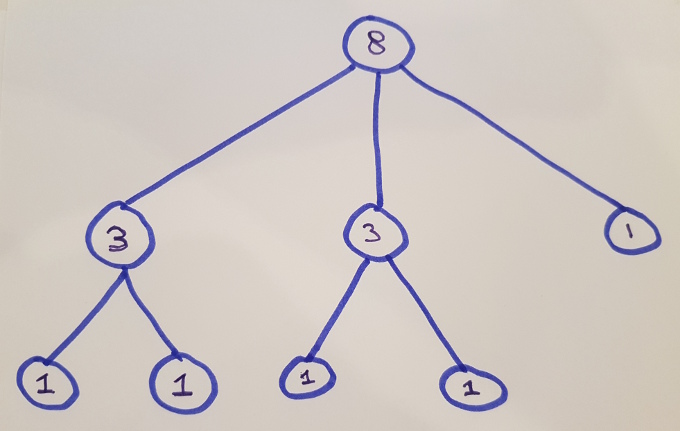
To see this in action, consider the catamorphism of “total size” which is depicted graphically below. In this picture each node is annotated a size showing the total size of that subtree:

Replacing the right-most child of the root node is depicted below. A red arrow with an “R” depicts the replacing of one node by another; Green arrows depict the fact that recalculation at the root node considers the values at that node’s direct children; a 9 at the root represents the updated outcome of the calculation.

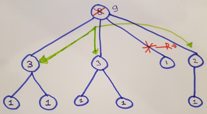
The fact that no green arrows point at the leaf-nodes on the bottom left represents the efficiency-gain with respect to a full recalculation of the catamorphism on the new input structure.

In this example, the effect is not all too dramatic, because the tree is relatively small; in the general case, dramatic efficiency gains will be made precisely when they are required, namely when the trees are very large.

Performance characteristics

Let us explore the computational cost of a single modification. This cost is built up from two separate parts:

1. Recursively constructing a new child.
2. Combining the results of the children.

Recursive construction

We start by considering the cost of recursively computing the result for a new child.

Note that for Delete there is no new child, and hence there is no cost. Insert and Replace both take as one of their parameters a history: a sequence of modifications.

The cost of recursive construction of a child is then: the sum of the costs for each modification in this history. That is to say: the cost of the step-wise recursive application of the algorithm. The cost of a each modification in the history is thus recursively described by the section “Performance characteristics” of this article.

The other factor is the length of the history for which recalculations must be done.

In the case of a Replace it is the number of new items in the provided history at least if we apply the constraint that replace can only replace with a continuation of the existing history. That is because only for new items in the provided history recalculations need to be done.

In the case of Insert this is the full length of the provided history: no earlier result is available, so we must calculate from scratch.

Combining results: the algebra

The computational cost of each call to the algebra depends on the algebra at hand.

Let’s consider two examples with rather different computational complexity to see how this is the case:

A first example is the summation of values shown at the beginning of this article. It scales linearly with the number of children (branching factor). This is because while taking the sum over all children we must consider each child at least once.

Contrast this with the serialization of a data structure into a single piece of contiguous memory. That scales linearly with the sum of the child result lengths (which is the same as to say: scales linearly with the output’s length). This is because each serialized child needs to be fully included in the result. Copying each child takes a time linear with the child’s size.

Now let’s consider how the computational cost of the algebra affects the computational cost of the algorithm as a whole. For the algorithm of selective recalculation of a catamorphic function outlined above, the computational cost of the algebra is recursively incurred at each level of the tree. For algebras that have a computational cost that is linear with the branching factor, such as the sum-of-values, this means that the total cost is in the order of the product of the following 3 things:

• The average branching factor of the tree
• The depth of the tree (more precisely: the deepest level where modification takes place)
• The number of modifications at the deepest level.

For large trees with small modifications this implies a great efficiency gain in comparison to a full recalculation.

Note that the above total cost of the algorithm is only applicable when the cost of the algebra is linear with the branching factor.

Serialization into contiguous memory, as detailed above, is an important example of this condition not holding. As a result, it is better not to implement it using selective recalculation. Recalculation from scratch at each step is significantly cheaper.

Incremental calculation of algebras

In the above approach, the performance gains with respect to a full recalculation are made by selectively recursing: results that are already known are not recalculated.

However, the result of the algebraic function is calculated precisely as in the non-incremental case: at each node at which recalculation takes place we do a full recomputation of the algebraic function with all its inputs.

For each such recomputation, the branching factor forms a lower bound on the performance: the inputs must at least be collected and passed to the algebra, and each child forms an input. For the algorithm as a whole, this lower bound is reflected as one of the 3 factors mentioned in the bulleted list above.

This raises the question: is it possible to arrive at the result of the algebraic function without considering all its inputs?

Let us revisit the example of total tree-size, as mentioned above, to see how the answer to that question may be “yes”.

Consider again the graphical example in the above. In it, a node with a total size of 1 is replaced with a node with a value of 2. From this fact alone, we can conclude that the total tree size is increased by 1 (namely: 2 - 1). Using the knowledge that the previous tree size was 8, we can conclude that the new tree size will be 9. This conclusion can be reached without referring to the two existing nodes with value 3. In other words: the branching factor does not come into play.

In general, we may sometimes have access to a mechanism of recalculation of the algebraic function that is not bound by the branching factor. This is made possible by taking a previous result of the algebraic function, as well as structred updates (deletions, insertions, replacements), into account. In other words: such mechanisms take an incremnental approach to the algebraic function.

In general, such a mechanism will always be available for a given catamorphism given two conditions:

• The outcome of combining results is unaffected the order of the children. (An example of this condition not holding: propagation of the left-most symbol occurring in a tree to its root)
• The effect of removing a single child can be expressed without taking into account the other children. (An example of this condition not holding: calculating the set of unique symbols)

Conclusion

In this article we have taken a look at catamorphisms in the context of controlled modification.

Some recursive functions can be expressed as a catamorphism. If the computational complexity of the associated algebra scales sub-linearly with the size of the underlying tree, an algorithm for efficient stepwise recalculation is available.

For some algebras we can do even better: we can ignore the values of the presently existing children entirely, and calculate a new value based purely by applying the results of deletion and insertion.